Introduction
Welcome to Data & AI Bootkon!
Data & AI Bootkon is an immersive hackathon designed for tech enthusiasts, developers, and innovators to explore the power of Google Cloud products through hands-on learning. This event provides a unique, integrated experience using Google Cloud Shell tutorials, enabling participants to dive deep into cutting-edge cloud technologies.
This event is comprised of the following code labs:
| Duration | Topic | Details |
|---|---|---|
| 30min | Environment Setup | Log into your GCP account and set up your environment. |
| 45min | Data Ingestion | Ingest data using three different methods: BigLake, Pub/Sub, and DataProc |
| 45min | Dataform | Create version-controlled SQL workflows for BigQuery |
| 60min | Machine Learning | Train a model on fraud detection and create an automated ML pipeline |
| 60min | Dataplex | Data governance at scale using Dataplex |
You can navigate this handbook using the < and > buttons on the right and left hand side, respectively. To get started, please press the > button on the right hand side now.
Use Case
Your role: As a senior data analytics/AI engineer at an imaginary company called FraudFix Technologies, you will tackle the challenges of making financial transactions safer using machine learning. Your work will involve analyzing vast amounts of transaction data to detect and prevent fraud, as well as assessing customer sentiment regarding the quality of transaction services. You will leverage a unique dataset, which includes auto-generated data by Google Gemini and public European credit card transactions that have been PCA transformed and anonymized. This dataset will be used to train your models, reflecting real-world applications of GCP Data & AI in enhancing financial safety.

Data Sources.
You’ll start by working with raw data that comes in different formats (csv , parquets).
Those data files are stored in a github repository. Your first task is to store the raw data into your Google Cloud Storage (GCS) bucket.
Data Ingestion Layer
You will bring this data into your BigQuery AI Lakehouse environment.
For batch data, you’ll use Dataproc Serverless and BigLake.
For near real-time data, you’ll use Pub/Sub to handle data as it comes in.
Because we want to simulate data ingestion at scale, we will be using the raw data that you have stored in GCS to simulate both batch and real time ingestion.
These tools help you get the data ready for processing and analysis.
BigQuery AI Lakehouse Think of this as the main camp where all your data hangs out. It’s a GCP product called BigQuery, and it’s designed to work with different types of data, whether it’s structured neatly in tables or unstructured like a pile of text documents. Here, you can run different data operations without moving data around.
Data Governance Layer This is where you ensure that your data is clean, secure, and used properly. Using Dataplex, you’ll set rules and checks to maintain data quality and governance.
Consumption Layer
Once you have your insights, you’ll use tools like Vertex AI for machine learning tasks and Looker Studio for creating reports and dashboards. This is where you turn data into something valuable, like detecting fraud or understanding customer sentiment.
Your goal is to share the results of your data predictions to your customers in a secure and private way. You will be using Analytics Hub for data sharing.
Throughout the event, you’ll be moving through these layers, using each tool to prepare, analyze, and draw insights from the data. You’ll see how they all connect to make a complete data analytics workflow on the cloud.
About the data set
The datasets contain transactions made by credit cards in September 2013 by European cardholders, but also augmented by Google Gemini. This dataset presents transactions that occurred over two days, where there are a few hundred fraudulent transactions out of hundreds of thousands of transactions. It is highly unbalanced, with the positive class (frauds) accounting for less than 0.1% of all transactions (subject to testing in your notebooks). It contains only numeric input V* variables which are the result of a PCA transformation. Due to confidentiality issues, the owner of the dataset cannot provide the original features and more background information about the data.
Features V1, V2, … V28 are the principal components obtained with PCA, the only features which have not been transformed with PCA are ‘Time’ , ‘Feedback’ and ‘Amount’.
Feature ‘Time’ contains the seconds elapsed between each transaction and the first transaction in the dataset. Feature ‘Amount’ is the transaction Amount, this feature can be used for example-dependent cost-sensitive learning. Feature ‘Class’ is the response variable and it takes value 1 in case of fraud and 0 otherwise. Feature ‘Feedback’ represents customer selection on service quality after submitting the transaction. This feature has been auto-generated by Google Gemini and added to the original dataset.
During your machine learning experimentation using notebooks, one of the notebook cells will add your Google cloud account email address into the prediction dataset for traceability. This email address is treated as PII data and should not be shared externally outside of Fraudfix. The original dataset has been collected and analyzed during a research collaboration of Worldline and the Machine Learning Group of ULB (Université Libre de Bruxelles) on big data mining and fraud detection. If you need more details on current and past projects on related topics are available here and here.
Logging into Google Cloud
caution
Please follow the below steps exactly as written. Deviating from them has unintended consequences.
Let us set your your Google Cloud Console. Please:
-
Open a new browser window in Incognito mode.
-
Open this handbook in your newly opened incognito window and keep reading; close this window in your main browser window.
-
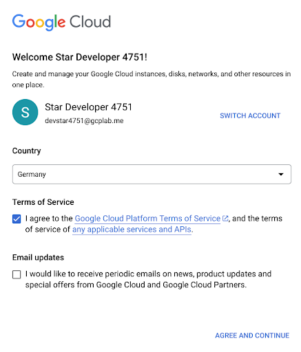
Open Google Cloud Console and log in with the provided credentials.
-
Accept the Terms of Services.
-
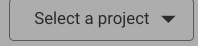
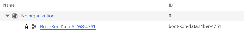
Choose your project id. Click on select a project and select the project ID (example below)
-
Go to language settings and change your language to
English (US). This will help our tutorial engine recognize items on your screen and make our table captain be able to help you.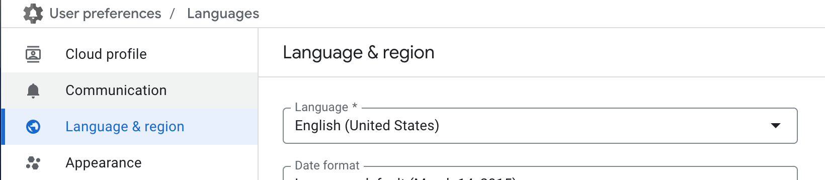
Executing code labs
During this event, we will guide you through a series of labs using Google Cloud Shell.
Cloud Shell is a fully interactive, browser-based environment for learning, experimenting, and managing Google Cloud projects. It comes preloaded with the Google Cloud CLI, essential utilities, and a built-in code editor with Cloud Code integration, enabling you to develop, debug, and deploy cloud apps entirely in the cloud.
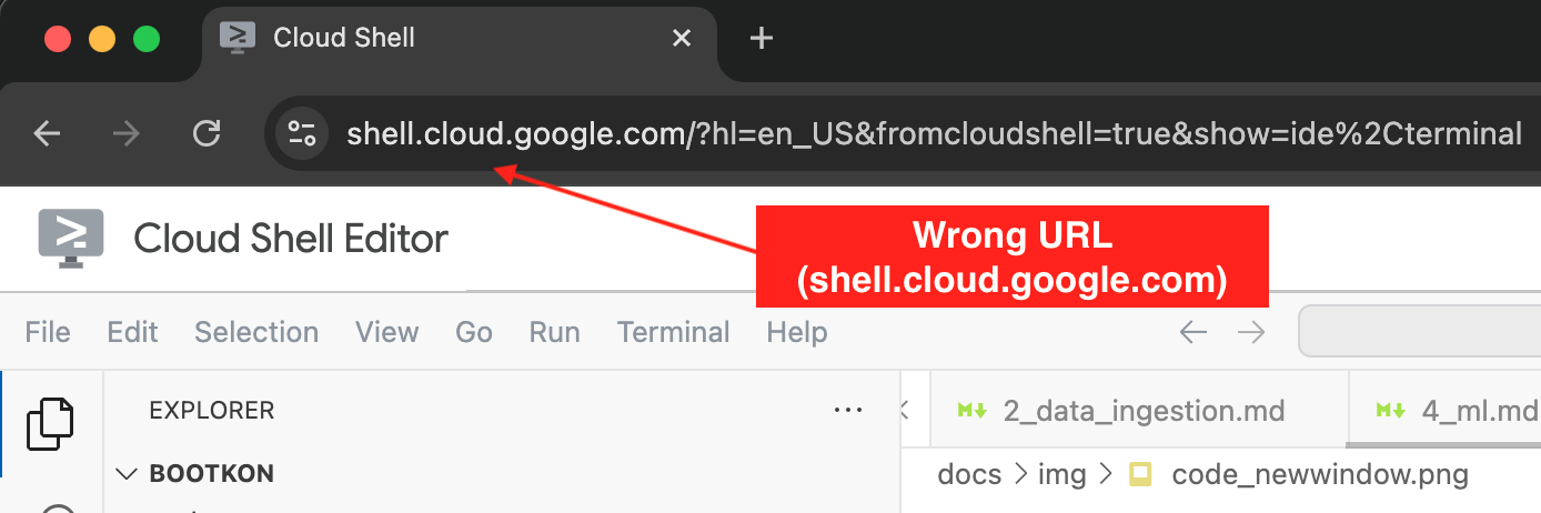
Below you can find a screenshot of Cloud Shell.
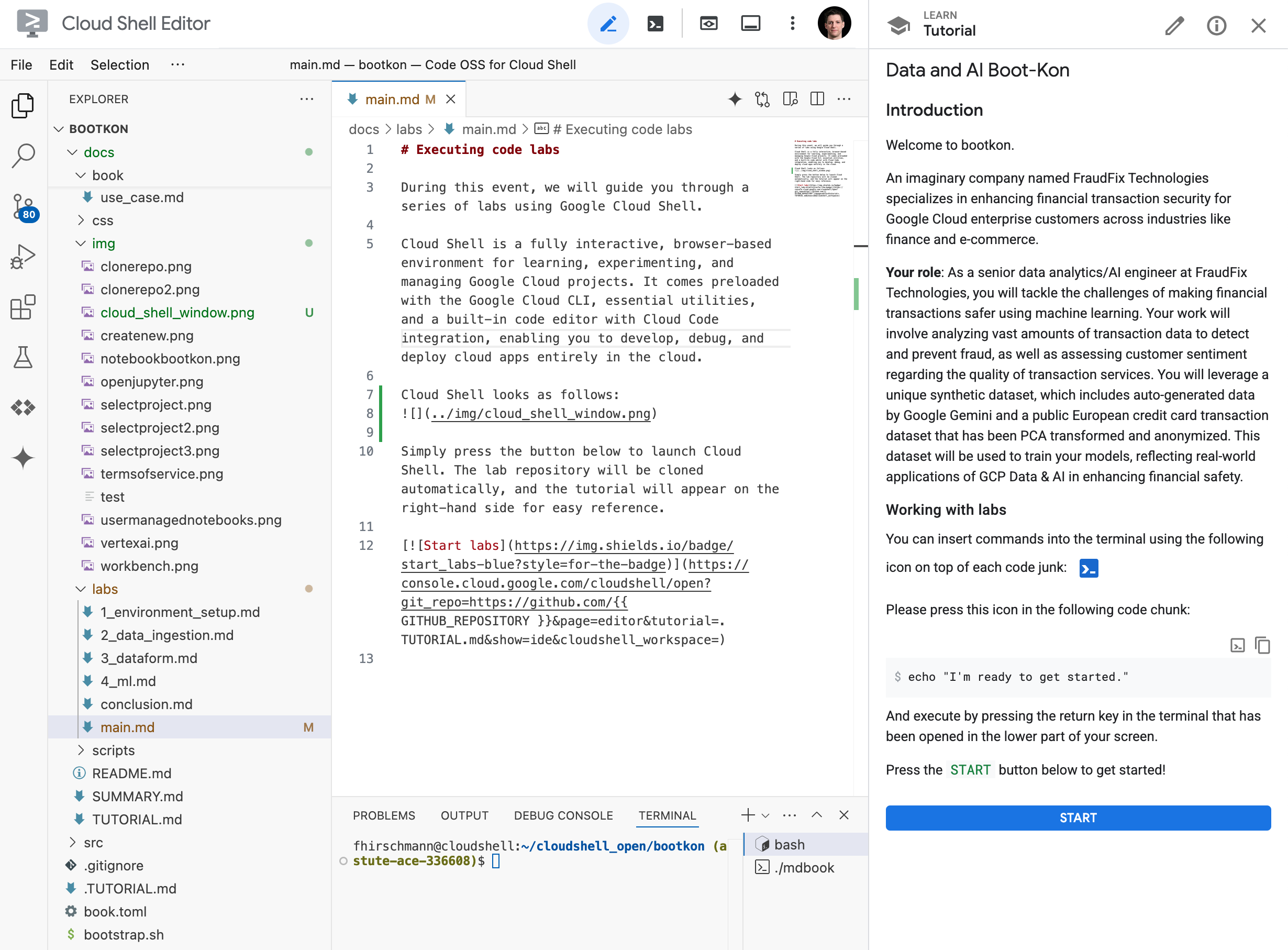
It is based on Visual Studio Code and hence looks like a normal IDE. However, on the right hand side you see the tutorial you will be working through. When you encouter code chunks in the tutorial, there are two icons on the right hand side. One to copy the code chunk to your clipboard and the other one to insert it directly into the terminal of Cloud Shell.
Working with labs (important)
Please note the points in this section before you get started with the labs in the next section.
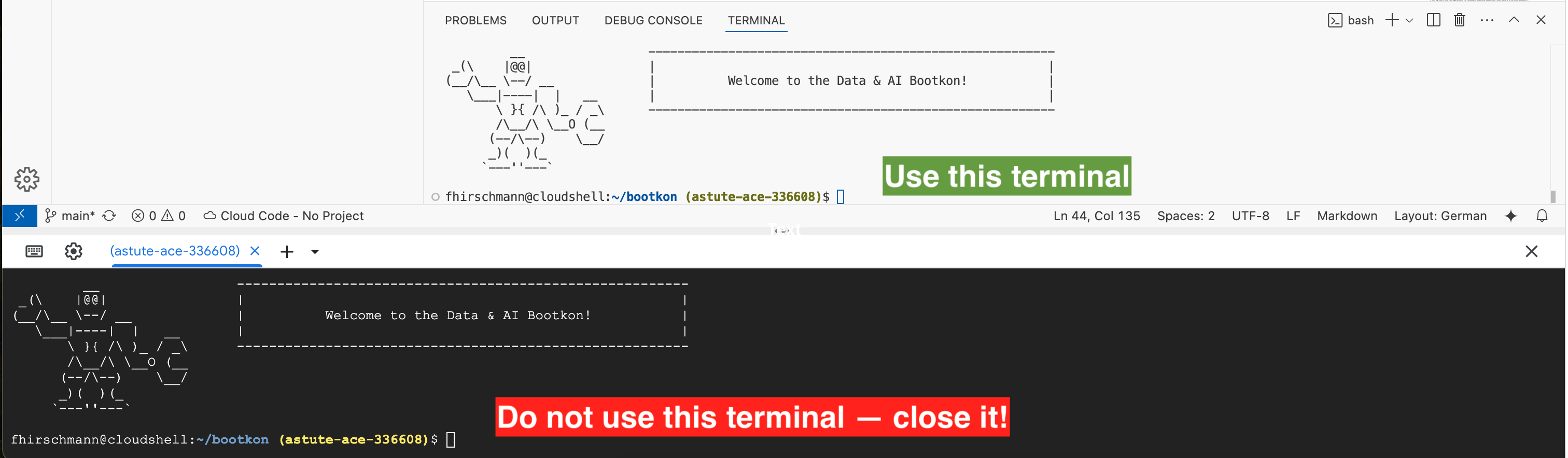
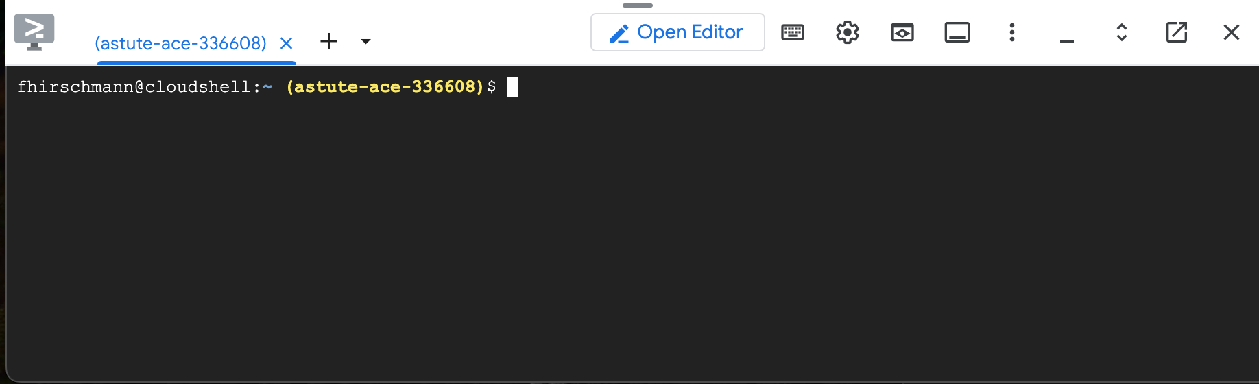
While going through the code labs, you will encounter two different terminals on your screen. Please only use the terminal from the IDE (white background) and do not use the non-IDE terminal (black background). In fact, just close the terminal with black background using the X button.
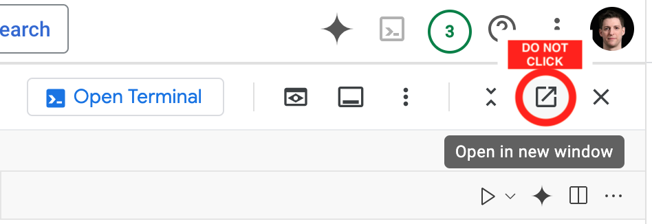
You will also find two buttons on your screen that might seem tempting. Please do not click the Open Terminal or Open in new window buttons as they will destroy the integrated experience of Cloud Shell.
Please double check that the URL in your browser reads console.cloud.google.com and not shell.cloud.google.com.
Should you accidentally close the tutorial or the IDE, just type the following command into the terminal:
bk-start
Start the lab
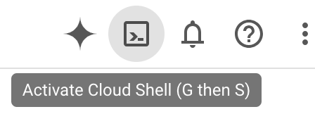
In your Google Cloud Console window (see the previous step), activate Cloud Shell.
Click into the terminal that has opened at the bottom of your screen.
And copy & paste the following command and press return:
BK_REPO=fhirschmann/bootkon; . <(wget -qO- https://raw.githubusercontent.com/fhirschmann/bootkon/main/.scripts/bk)
Now, please go back to Cloud Shell and continue with the tutorial that has been opened on the right hand side of your screen!
Lab 1: Environment Setup
caution
You are viewing this lab from the handbook. This lab is meant to be loaded as Cloud Shell tutorial. Please see the labs section on how to do so.
In this lab we will set up your environment, download the data set for this Bootkon, put it to Cloud Storage, and do a few other things.
Enable services
First, we need to enable some Google Cloud Platform (GCP) services. Enabling GCP services is necessary to access and use the resources and capabilities associated with those services. Each GCP service provides a specific set of features for managing cloud infrastructure, data, AI models, and more. Enabling them takes a few minutes.
Assign permissions
Execute the following script:
bk-bootstrap
But what did it do? Let’s ask Gemini while it is running.
-
Open
bk-bootstrap. -
Open Gemini Code Assist
-
Insert
What does bk-bootstrap do?into the Gemini prompt.
Cloud Shell may ask you to select your project and enable the API. Do not worry about missing licenses.
Download data
Next, we download the data set for Bootkon and put it into Cloud Storage. Before we do that, we create
a bucket where we place the data into. Let’s name it <PROJECT_ID>-bucket:
gsutil mb -l $REGION gs://<PROJECT_ID>-bucket
The next command will download the dataset from GitHub and extract it to Cloud Shell:
wget -qO - https://github.com/fhirschmann/bootkon-data/releases/download/v1.7.1/data.tar.gz | tar xvzf -
Let’s upload the data to the bucket we just created:
gsutil -m cp -R data gs://<PROJECT_ID>-bucket/
Is the data there? Let’s check and open Cloud Storage. Once you have checked, you may need to resize the window that just opened to make it smaller in case you run out of screen real estate.
Create default VPC
The Google Cloud environment we created for you does not come with a Virtual Private Cloud (VPC) network created by default. Let’s create one. If it already exists – that’s ok.
gcloud compute networks create default --project=$PROJECT_ID --subnet-mode=auto --bgp-routing-mode="regional"
Let’s also create/update the subnet to allow internal traffic:
gcloud compute networks subnets update default --region=$REGION --enable-private-ip-google-access
If the command above returned an error about a visibility check, please wait two minutes for the permissions to propagate and try again.
Next, create a firewall rule:
gcloud compute firewall-rules create "default-allow-all-internal" \
    --network="default" \
    --project=$PROJECT_ID \
    --direction=INGRESS \
    --priority=65534 \
    --source-ranges="10.128.0.0/9" \
    --allow=tcp:0-65535,udp:0-65535,icmp
Success
🎉 Congratulations! You’ve officially leveled up from “cloud-curious” to “GCP aware”! 🌩️🚀
Lab 2: Data Ingestion
caution
You are viewing this lab from the handbook. This lab is meant to be loaded as Cloud Shell tutorial. Please see the labs section on how to do so.
Welcome back 😍!
During this lab, you ingest fraudulent and non fraudulent transactions into BigQuery using three methods:
- Method 1: Using BigLake with data stored in Google Cloud Storage (GCS)
- Method 2: Near real-time ingestion into BigQuery using Cloud Pub/Sub
- Method 3: Batch ingestion into BigQuery using Dataproc Serverless
For all methods, we are ingesting data from the bucket you have created in the previous lab.
Method 1: External table using BigLake
BigLake tables allow querying structured data in external data stores with access delegation. For an overview, refer to the BigLake documentation. Access delegation decouples access to the BigLake table from access to the underlying data store. An external connection associated with a service account is used to connect to the data store.
Because the service account handles retrieving data from the data store, you only have to grant users access to the BigLake table. This lets you enforce fine-grained security at the table level, including row-level and column-level security.
First, we create the connection resource in BigQuery:
bq mk --connection --location=us --project_id=<PROJECT_ID> \
    --connection_type=CLOUD_RESOURCE fraud-transactions-conn
When you create a connection resource, BigQuery creates a unique system service account and associates it with the connection.
bq show --connection <PROJECT_ID>.us.fraud-transactions-conn
Note the serviceAccountID.
To connect to Cloud Storage, you must give the new connection read-only access to Cloud Storage so that BigQuery can access files on behalf of users. Let’s assign the service account to a variable:
CONN_SERVICE_ACCOUNT=$(bq --format=prettyjson show --connection ${PROJECT_ID}.us.fraud-transactions-conn | jq -r ".cloudResource.serviceAccountId")
echo $CONN_SERVICE_ACCOUNT
Let’s double check the service account.
- Go to the BigQuery Console.
- Click
Explorer - Expand
<PROJECT_ID> - Click
Connections - Click
fraud-transactions-conn
Is the service account equivalent to the one you got from the command line?
If so, let’s grant the service account access to Cloud Storage:
gcloud storage buckets add-iam-policy-binding gs://<PROJECT_ID>-bucket \
--role=roles/storage.objectViewer \
--member=serviceAccount:$CONN_SERVICE_ACCOUNT
Let’s create a data set that contains the table and the external connection to Cloud Storage.
- Go to the BigQuery Console
- Choose
Explorer - Hover your mouse over
<PROJECT_ID> - Click the three vertical dots (⋮) and go to
Create dataset - Enter
ml_datasets(plural) in the ID field. Region should be multi-region US. - Click
Create dataset
Alternatively, you can create the data set on the command line:
bq --location=us mk -d ml_datasets
Next, we connect the data in Cloud Storage to BigQuery:
- Choose
Explorer - Click
+ Add data - Click
Google Cloud Storage - Select
Load to BigQuery - Enter the following details:
- Create table from:
Google Cloud Storage - Select file:
<PROJECT_ID>-bucket/data/parquet/ulb_fraud_detection/* - File format:
Parquet - Project:
<PROJECT_ID> - Dataset:
ml_datasets - Table:
ulb_fraud_detection_biglake - Table type:
External table - Check Create a BigLake table using a Cloud Resource connection
- Connection ID: Select
us.fraud-transactions-conn - Schema:
Auto detect
- Click on
Create table
Alternatively, you can also use the command line to create the table:
bq mk --table \
  --external_table_definition=@PARQUET="gs://${PROJECT_ID}-bucket/data/parquet/ulb_fraud_detection/*"@projects/${PROJECT_ID}/locations/us/connections/fraud-transactions-conn \
  ml_datasets.ulb_fraud_detection_biglake
Let’s have a look at the data set:
- Go to the BigQuery Console
- Choose
Explorer - Expand
<PROJECT_ID> - Click
Datasets - Click
ml_datasets - Click
ulb_fraud_detection_biglake - Click
Details
Have a look at the external data configuration. You can see the Cloud Storage bucket (gs://...) your data
lives in.
Let’s query it:
- Click
Query - Insert the following SQL query.
SELECT * FROM `<PROJECT_ID>.ml_datasets.ulb_fraud_detection_biglake` LIMIT 1000;
Note that you can also execute a query using the bq tool:
bq --location=us query --nouse_legacy_sql "SELECT Time, V1, Amount, Class FROM <PROJECT_ID>.ml_datasets.ulb_fraud_detection_biglake LIMIT 10;"
The data you are querying still resides on Cloud Storage and there are no copies stored in BigQuery. When using BigLake, BigQuery acts as query engine but not as storage layer.
Method 2: Real time data ingestion into BigQuery using Pub/Sub
Pub/Sub enables real-time streaming into BigQuery. Learn more about Pub/Sub integrations with BigQuery.
We create an empty table and then stream data into it. For this to work, we need to specify a schema. Have a look at fraud_detection_bigquery_schema.json. This is the schema we are going to use.
Create an empty table using this schema. We will use it to stream data into it:
bq --location=us mk --table \
<PROJECT_ID>:ml_datasets.ulb_fraud_detection_pubsub src/data_ingestion/fraud_detection_bigquery_schema.json
We also need to create a Pub/Sub schema. We use Apache Avro, as it is better suited for appending row-wise:
gcloud pubsub schemas create fraud-detection-schema \
    --project=$PROJECT_ID  \
    --type=AVRO \
    --definition-file=src/data_ingestion/fraud_detection_pubsub_schema.json
And then create a Pub/Sub topic using this schema:
gcloud pubsub topics create fraud-detection-topic \
    --project=$PROJECT_ID  \
    --schema=fraud-detection-schema \
    --message-encoding=BINARY
We also need to give Pub/Sub permissions to write data to BigQuery. The Pub/Sub service account is created automatically and
is comprised of the project number (not the id) and an identifier. In your case, it is service-<PROJECT_NUMBER>@gcp-sa-pubsub.iam.gserviceaccount.com
And grant the service account access to BigQuery:
gcloud projects add-iam-policy-binding $PROJECT_ID \
    --member=serviceAccount:service-<PROJECT_NUMBER>@gcp-sa-pubsub.iam.gserviceaccount.com --role=roles/bigquery.dataEditor

gcloud projects add-iam-policy-binding $PROJECT_ID \
    --member=serviceAccount:service-<PROJECT_NUMBER>@gcp-sa-pubsub.iam.gserviceaccount.com --role=roles/bigquery.jobUser
Next, we create the Pub/Sub subscription:
gcloud pubsub subscriptions create fraud-detection-subscription \
    --project=$PROJECT_ID  \
    --topic=fraud-detection-topic \
    --bigquery-table=$PROJECT_ID.ml_datasets.ulb_fraud_detection_pubsub \
    --use-topic-schema
Examine it in the console:
- Go to the Pub/Sub Console
- Click
fraud-detection-subscription . Here you can see messages as they arrive. - Click
fraud-detection-topic . This is the topic you will be publishing messages to.
Please have a look at import_csv_to_bigquery_1.py. This script loads CSV files from Cloud Storage, parses it in Python, and sends it to Pub/Sub - row by row.
Let’s execute it.
./src/data_ingestion/import_csv_to_bigquery_1.py
Each line you see on the screen corresponds to one transaction being sent to Pub/Sub and written to BigQuery. It would take approximately 40 to 60 minutes for it to finish. So, please cancel the command using CTRL + C.
But why is it so slow?
Let’s ask Gemini:
-
Open Gemini Code Assist
-
Insert
Why is import_csv_to_bigquery_1.py so slow?into the Gemini prompt.
Method 3: Ingestion using Cloud Dataproc (Apache Spark)
Dataproc is a fully managed and scalable service for running Apache Hadoop, Apache Spark, Apache Flink, Presto, and 30+ open source tools and frameworks. Dataproc allows data to be loaded and also transformed or pre-processed as it is brought in.
Create an empty BigQuery table:
bq --location=us mk --table \
<PROJECT_ID>:ml_datasets.ulb_fraud_detection_dataproc src/data_ingestion/fraud_detection_bigquery_schema.json
Download the Spark connector for BigQuery and copy it to our bucket:
wget -qN https://github.com/GoogleCloudDataproc/spark-bigquery-connector/releases/download/0.37.0/spark-3.3-bigquery-0.37.0.jar
gsutil cp spark-3.3-bigquery-0.37.0.jar gs://${PROJECT_ID}-bucket/jar/spark-3.3-bigquery-0.37.0.jar
Open <PROJECT_ID>. Don’t forget to save.
Execute it:
gcloud dataproc batches submit pyspark src/data_ingestion/import_parquet_to_bigquery.py \
    --project=$PROJECT_ID \
    --region=$REGION \
    --deps-bucket=gs://${PROJECT_ID}-bucket
While the command is still running, open the DataProc Console and monitor the job.
After the Dataproc job completes, confirm that data has been loaded into the BigQuery table. You should see over 200,000 records, but the exact count isn’t critical:
bq --location=us query --nouse_legacy_sql "SELECT count(*) as count FROM <PROJECT_ID>.ml_datasets.ulb_fraud_detection_dataproc;"
❗ Please do not skip the above validation step. Data in the above table is needed for the following labs.
Success
🎉 Congratulations! 🚀
You’ve officially leveled up in data wizardry! By conquering the BigQuery Code Lab, you’ve shown your skills in not just one, but three epic methods: BigLake (riding the waves of data), DataProc (processing like a boss), and Pub/Sub (broadcasting brilliance).
Your pipelines are now flawless, your tables well-fed, and your data destiny secured. Welcome to the realm of BigQuery heroes — the Master of Ingestion! 🦾💻
Lab 3: Dataform
caution
You are viewing this lab from the handbook. This lab is meant to be loaded as Cloud Shell tutorial. Please see the labs section on how to do so.
During this lab, you gather user feedback to assess the impact of model adjustments on real-world use (prediction), ensuring that our fraud detection system effectively balances accuracy with user satisfaction.
- Use Dataform, BigQuery and Gemini to Perform sentiment analysis of customer feedback.
Dataform
Dataform is a fully managed service that helps data teams build, version control, and orchestrate SQL workflows in BigQuery. It provides an end-to-end experience for data transformation, including:
- Table definition: Dataform provides a central repository for managing table definitions, column descriptions, and data quality assertions. This makes it easy to keep track of your data schema and ensure that your data is consistent and reliable.
- Dependency management: Dataform automatically manages the dependencies between your tables, ensuring that they are always processed in the correct order. This simplifies the development and maintenance of complex data pipelines.
- Orchestration: Dataform orchestrates the execution of your SQL workflows, taking care of all the operational overhead. This frees you up to focus on developing and refining your data pipelines.
Dataform is built on top of Dataform Core, an open source SQL-based language for managing data transformations. Dataform Core provides a variety of features that make it easy to develop and maintain data pipelines, including:
- Incremental updates: Dataform Core can incrementally update your tables, only processing the data that has changed since the last update.
- Slowly changing dimensions: Dataform Core provides built-in support for slowly changing dimensions, which are a common type of data in data warehouses.
- Reusable code: Dataform Core allows you to write reusable code in JavaScript, which can be used to implement complex data transformations and workflows.
Dataform is integrated with a variety of other Google Cloud services, including GitHub, GitLab, Cloud Composer, and Workflows. This makes it easy to integrate Dataform with your existing development and orchestration workflows.
Use Cases for Dataform
Dataform can be used for a variety of use cases, including:
- Data Warehousing: Dataform can be used to build and maintain data warehouses that are scalable and reliable.
- Data Engineering: Dataform can be used to develop and maintain data pipelines that transform and load data into data warehouses.
- Data Analytics: Dataform can be used to develop and maintain data pipelines that prepare data for analysis.
- Machine Learning: Dataform can be used to develop and maintain data pipelines that prepare data for machine learning models.
Create a Dataform Pipeline
First step in implementing a pipeline in Dataform is to set up a repository and a development environment. Detailed quickstart and instructions can be found here.
Create a Repository in Dataform
Go to Dataform (part of the BigQuery console).
-
Click on
+ CREATE REPOSITORY -
Use the following values when creating the repository:
Repository ID:
hackathon-repository
Region:us-central1
Service Account:Default Dataform service account -
Set actAs permission checks to
Don't enforce -
And click on
CREATE The dataform service account you see on your screen should be
service-<PROJECT_NUMBER>@gcp-sa-dataform.iam.gserviceaccount.com. We will need it later. -
Select
Grant all required roles for the service-account to execute queries in Dataform
Next, click
Create a Dataform Workspace
You should now be in the
First, click
In the Create development workspace window, do the following:
-
In the
Workspace ID field, enterhackathon--workspaceor any other name you like. -
Click
CREATE -
The development workspace page appears.
-
Click on the newly created
hackathon--workspace -
Click
Initialize workspace
Adjust workflow settings
We will now set up our custom workflow.
-
Edit the
workflow_settings.yamlfile : -
Replace
defaultDatasetvalue withml_datasets -
Make sure
defaultProjectvalue is<PROJECT_ID> -
Click on
INSTALL PACKAGES only once. You should see a message at the bottom of the page:Package installation succeeded
Next, let’s create several workflow files.
-
Delete the following files from the
*definitions folder:first_view.sqlxsecond_view.sqlx -
Within
*definitions create a new directory calledmodels:
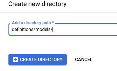
-
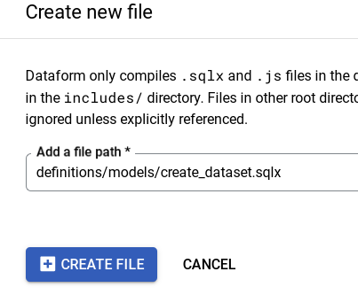
Click on
modelsdirectory and create 2 new filescreate_dataset.sqlxllm_model_connection.sqlxExample:
-
Copy the contents to each of those files:
-
Click on
*definitions and create 3 new files:mview_ulb_fraud_detection.sqlxsentiment_inference.sqlxulb_fraud_detection.sqlx
Example:

-
Copy the contents to each of those files:
-
Set the
databasevalue to your project ID<PROJECT_ID>value inulb_fraud_detection.sqlxfile:

- In
llm_model_connection.sqlx, replace theus.llm-connectionconnection with the connection name you have created in LAB 2 during the BigLake section. If you have followed the steps in LAB 2, the connected name should beus.fraud-transactions-conn
Notice the usage of $ref in line 11, of definitions/mview_ulb_fraud_detection.sqlx. The advantages of using $ref in Dataform are
- Automatic Reference Management: Ensures correct fully-qualified names for tables and views, avoiding hardcoding and simplifying environment configuration.
- Dependency Tracking: Builds a dependency graph, ensuring correct creation order and automatic updates when referenced tables change.
- Enhanced Maintainability: Supports modular and reusable SQL scripts, making the codebase easier to maintain and less error-prone.
Execute Dataform workflows
Run the dataset creation by Tag. Tag allow you to just execute parts of the workflows and not the entire workflow.
Note: If you have previously granted all required roles for the service account service-<PROJECT_NUMBER>@gcp-sa-dataform.iam.gserviceaccount.com then you can skip step 1-5
-
Click on
Start execution >Tags >dataset_ulb_fraud_detection_llm At the top where it says “Authentication”, make sure you select
Execute with selected service accountand choose your dataform service account:service-<PROJECT_NUMBER>@gcp-sa-dataform.iam.gserviceaccount.comThen click
Start execution -
Click on
DETAILS Notice the Access Denied error on BigQuery for the dataform service account
service-<PROJECT_NUMBER>@gcp-sa-dataform.iam.gserviceaccount.com. If did not receive an error, you can skip step 3-6. -
Go to IAM & Admin
-
Click on
GRANT ACCESS and grantBigQuery Data Editor , BigQuery Job User and BigQuery Connection Userto the principalservice-<PROJECT_NUMBER>@gcp-sa-dataform.iam.gserviceaccount.com. -
Click on
SAVE

Note: If you encounter a policy update screen, just click on update.
-
Go back to Dataform within in BigQuery, and retry
Start execution >Tags >dataset_ulb_fraud_detection_llm At the top where it says “Authentication”, make sure you select
Execute with selected service accountand choose your dataform service account:service-<PROJECT_NUMBER>@gcp-sa-dataform.iam.gserviceaccount.comThen click
Start execution
Notice the execution status. It should be a success. -
Lastly, go to Compiled graph and explore it. Go to Dataform>
hackathon-repository >hackathon--workspace>COMPILED GRAPH
Execute the workspace workflow
For the sentiment inference step to succeed, you need to grant the external connection service account the Vertex AI user privilege. More details can be found in this link.
- You can find the service account ID under BigQuery Studio >
Explorer ><PROJECT_ID>>Connections >fraud-transactions-conn

-
Take note of the service account and grant it the
Vertex AI Userrole in IAM.

-
Back in your Dataform workspace, click
Start execution from the top menu, thenExecute Actions At the top where it says “Authentication”, make sure you select
Execute with selected service accountand choose your dataform service account:service-<PROJECT_NUMBER>@gcp-sa-dataform.iam.gserviceaccount.com -
Click on
ALL ACTIONS Tab followed by choosingStart execution -
Check the execution status. It should be a success.
-
Verify the new table
sentiment_inferencein theml_datasetsdataset in BigQuery and query the BigQuery table content (At this point you should be familiar with running BigQuery SQL)SELECT distinct ml_generate_text_llm_result, prompt, Feedback FROM `ml_datasets.sentiment_inference` LIMIT 10;[Max 2 minutes] Discuss the table results within your team group.
-
Before moving to the challenge section of the lab, go back to the
Code section of the Dataform workspace. At the top of the “Files” section on the left, clickCommit X Changes (X should be about 7), add a commit message like, “Bootkon lab 3”, then clickCommit all files and thenPush to default branch You should now have the message: Workspace is up to date
Challenge section: production, scheduling and automation
Automate and schedule the compilation and execution of the pipeline. This is done using release configurations and workflow configurations.
Release Configurations:
Release configurations allow you to compile your pipeline code at specific intervals that suit your use case. You can define:
-
Branch, Tag, or Commit SHA: Specify which version of your code to use.
-
Frequency: Set how often the compilation should occur, such as daily or weekly.
-
Compilation Overrides: Use settings for testing and development, such as running the pipeline in an isolated project or dataset/table.
Common practice includes setting up release configurations for both test and production environments. For more information, refer to the release configuration documentation.
Workflow Configurations
To execute a pipeline based on your specifications and code structure, you need to set up a workflow configuration. This acts as a scheduler where you define:
-
Release Configuration: Choose the release configuration to use.
-
Frequency: Set how often the pipeline should run.
-
Actions to Execute: Specify what actions to perform during each run.
The pipeline will run at the defined frequency using the compiled code from the specified release configuration. For more information, refer to the workflow configurations documentation.
[TASK] Challenge : Take up to 10 minutes to Setup a Daily Frequency Execution of the Workflow
Goal: Set up a daily schedule to automate and execute the workflow you created.
- Automate and schedule the pipeline’s compilation and execution.
- Define release configurations for one production environment (optionally: you can create another one for dev environment)
- Set up workflow configurations to schedule pipeline execution (use dataform service account).
- Set up a 3 minute frequency execution of the workflow you have created.
Note: If you are stuck and cannot figure out how to proceed after a few minutes, ask your team captain.
Success
🎉 Congratulations! 🚀
You’ve just finished the lab, and wow, what a ride! You dove headfirst into the world of Dataform, BigQuery, and Gemini, building a sentiment analysis pipeline from scratch. Remember all those setup steps? Repository, workspace, connections…it’s a blur now, but you nailed it.
Those pesky “Access Denied” errors? Conquered. The pipeline? Purring like a data-driven kitten, churning out sentiment scores like nobody’s business. And the best part? You automated the whole thing! Scheduled executions? Check. You’re a data pipeline master. Bring on the next challenge – you’ve got this! 🚀
Lab 4: ML Operations
caution
You are viewing this lab from the handbook. This lab is meant to be loaded as Cloud Shell tutorial. Please see the labs section on how to do so.
In this lab, we will build a machine learning model to assess, in real-time, whether incoming transactions are fraudulent or legitimate. Using Vertex AI Pipelines (based on Kubeflow), we will streamline the end-to-end ML workflow, from data preprocessing to model deployment, ensuring scalability and efficiency in fraud detection.
In Vertex AI, custom containers allow you to define and package your own execution environment for machine learning workflows. To store custom container images, create a repository in artifact registry:
gcloud artifacts repositories create bootkon --repository-format=docker --location=us-central1
Let us create two container images, one for training and one for serving predictions.
The training container is comprised of the following files. Please have a look at them:
train/Dockerfile: Executes the training script.train/train.py: Downloads the data set from BigQuery, trains a machine learning model, and uploads the model to Cloud Storage.
The serving container image is comprised of the following files:
predict/Dockerfile: Executes the serving script to answer requests.predict/predict.py: Downloads the model from Cloud Storage, loads it, and answers predictions on port8080.
We can create the container images using Cloud Build, which allows you to build a Docker image using just a Dockerfile. The next command builds the image in Cloud Build and pushes it to Artifact Registry:
(cd src/ml/train && gcloud builds submit --region=us-central1 --tag=us-central1-docker.pkg.dev/<PROJECT_ID>/bootkon/bootkon-train:latest --quiet)
Let’s do the same for the serving image:
(cd src/ml/predict && gcloud builds submit --region=us-central1 --tag=us-central1-docker.pkg.dev/<PROJECT_ID>/bootkon/bootkon-predict:latest --quiet)
Vertex AI Pipelines
Now, have a look at pipeline.py. This script uses the Kubeflow domain specific language (dsl) to orchestrate the following machine learning workflow:
CustomTrainingJobOptrains the model.ModelUploadOpuploads the trained model to the Vertex AI model registry.EndpointCreateOpcreates a prediction endpoint for inference.ModelDeployOpdeploys the model from step 2 to the endpoint from step 3.
Let’s execute it:
python src/ml/pipeline.py
The pipeline run will take around 20 minutes to complete. While waiting, please read the introduction to Vertex AI Pipelines.
Custom Training Job
The pipeline creates a custom training job – let’s inspect it in the Cloud Console once it has completed:
- Open Vertex AI Console
- Click
Training in the navigation menu - Click
Custom jobs - Click
bootkon-training-job
Note the container image it uses and the arguments that are passed to the container (dataset in BigQuery and project id).
Model Registry
Once the training job has finished, the resulting model is uploaded to the model registry. Let’s have a look:
- Click
Model Registry in the nevigation menu - Click
bootkon-model - Click
VERSION DETAILS
Here you can can see that a model in the Vertex AI Model Registry is made up from a Container image as well as a Model artifact location. When you deploy a model, Vertex AI simply starts the container and points it to the artifact location.
Endpoint for Predictions
The endpoint is created in a parallel branch in the pipeline you just ran. You can deploy models to an endpoint through the model registry.
- Click
Endpoints in the navigation menu - Click
bootkon-endpoint
You can see that the endpoint has one model deployed currently, and all the traffic is routed to it (traffic split is 100%). When scrolling down, you get live graphs as soon as predictions are coming in.
You can also train and deploy models on Vertex in the UI only. Let’s have a more detailed look. Click
Vertex AI Pipelines
Let’s have a look at the Pipeline as well.
- Click
Pipelines in the navigation menu - Click
bootkon-pipeline-…
You can now see the individual steps in the pipeline. Please click through the individual steps of the pipeline and have a look at the Pipeline run analysis on the right hand side as you cycle pipeline steps.
Click on Expand Artifacts. Now, you can see expanded yellow boxes. These are Vertex AI artifacts that are created as a result of the previous step.
Feel free to explore the UI in more detail on your own!
Making predictions
Now that the endpoint has been deployed, we can send transactions to it to assess whether they are fraudulent or not.
We can use curl to send transactions to the endpoint.
Have a look at predict.sh. In line 9 it uses curl to call the endpoint using a data file named instances.json containing 3 transactions.
Let’s execute it:
./src/ml/predict.sh
The result should be a JSON object with a prediction key, containing the predictions for each of the 3 transactions. 1 means fraud and 0 means non-fraud.
Success
Congratulations, intrepid ML explorer! 🚀 You’ve successfully wrangled data, trained models, and unleashed the power of Vertex AI. If your model underperforms, remember: it’s not a bug—it’s just an underfitting feature! Keep iterating, keep optimizing, and may your loss functions always converge. Happy coding! 🤖✨
Lab 5: Data Governance with Dataplex
caution
You are viewing this lab from the handbook. This lab is meant to be loaded as Cloud Shell tutorial. Please see the labs section on how to do so.
In this lab you will
- Understand Dataplex product capabilities.
- Leverage Dataplex to understand and govern your data and metadata.
- Build data quality checks on top of the fraud detection prediction results.
About Dataplex
Dataplex is a data governance tool which helps you organize your data assets by overlaying the organizational concept of “Lakes” and “Zones”. This organization is logical only and does not require any data movement. You can use lakes to define, for example, organizational boundaries (e.g. marketing lake/sales lake) or regional boundaries (i.e. US lake/ UK lake), while zones are used to group data within lakes by data readiness or by use cases (e.g. raw_zone/curated_zone or analytics_zone/data_science_zone).
Dataplex can also be used to build a data mesh architecture with decentralized data ownership among domain data owners.
Security - Cloud Storage/BigQuery
With Dataplex you can apply data access permissions using IAM groups across multiple buckets and BigQuery datasets by granting permissions at a lake or zone-level. It will do the heavy lifting of propagating desired policies and updating access policies of the buckets/datasets that are part of that lake or data zone.
Dataplex will also apply those permissions to any new buckets/datasets that get created under that data zone. This takes away the need to manually manage individual bucket permissions and also provides a way to automatically apply permissions to any new data added to your lakes.
Note that the permissions are applied in “Additive” fashion - Dataplex does not replace the existing permissions when pushing down permissions. Dataplex also provides “exclusive” permission push down as an opt-in feature.
Discovery [semi-structured and structured data]
You can configure discovery jobs in Dataplex that can sample data on GCS, infer its schema, and automatically register it with the Dataplex Catalog so you can easily search and discover the data you have in your lakes.
In addition to registering metadata with Dataplex Catalog, for data in CSV, JSON, AVRO, ORC, and Parquet formats, the discovery jobs also register technical metadata, including hive-style partitions, with a managed Hive metastore (Dataproc Metastore) & as external tables in BigQuery (BQ).
Discovery jobs can be configured to run on a schedule to discover any new tables or partitions. For new partitions, discovery jobs incrementally scan new data, check for data and schema compatibility, and register only compatible schema to the Hive metastore/BQ so that your table definitions never go out of sync with your data.
Actions - Profiling, Quality, Lineage, Discovery
Dataplex has the capability to profile data assets (BigQuery tables), auto detect data lineage for BigQuery transformations. You can also use it for data discovery across GCS, BigQuery, Spanner, PubSub, Dataproc metastore, Bigtable and Vertex AI models.
You can automate the scanning of data, validate data against defined rules, and log alerts if your data doesn’t meet quality requirements. In addition you can manage data quality rules and deployments as code, improving the integrity of data production pipelines.
Create a Dataplex Lake
- Go to Dataplex.
- Navigate to
Manage . - Click
Create . - Enter the following details:
- Display name:
bootkon-lake - Description: anything you like
- Region:
us-central1 - Labels: Add labels to your lake. For example, use location for the key and berlin for the value over your data
- Metastore: lets skip the metastore creation for now
- Display name:
- Finally, click on
Create . This should take around 2-3 minutes.
Add Dataplex Zones
We will add two zones: one for raw data and another for curated data.
- Click on the
bootkon-lake lake you just created. - In the Zones tab, click
+ Add Zone and enter the following details:- Display name:
bootkon-raw-zone - Type: Raw Zone
- Description: anything you like
- Data Locations:
Regional (us-central1) - Discovery settings: Enable metadata discovery, which allows Dataplex to automatically scan and extract metadata from the data in your zone. Let’s leave the default settings. Set time zone to Germany.
- Display name:
Finally, click
Repeat the same steps but this time, change the display name to bootkon-curated-zone and choose Curated Zone for the Type. You might also change the label and description values.
The creation should take 2-3 minutes to finish.
Add Zone Data Assets
Let’s map data stored in Cloud Storage buckets and BigQuery datasets as assets in your zone.
- Navigate to Zones and click on
bootkon-raw-zone - Click
+ ADD ASSETS - Click
ADD AN ASSET - Choose Storage bucket from the type dropdown
- Display name :
bootkon-gcs-raw-asset - Optionally add a description
- Browse the bucket name and choose
<PROJECT_ID>-bucket. - Select the bucket
- Let’s skip upgrading to the managed option. When you upgrade a Cloud Storage bucket asset, Dataplex removes the attached external tables and creates BigLake tables. We have already created a BigLake table in Lab 2 so this option is not necessary.
- Optionally add a label
- Click
Continue - Leave the discovery setting to be inherited by the lake settings we have just created during lake creation steps. Click on
Continue . - Click
Submit .
Now let’s add another data asset but for the bootkon-curated-zone:
- Click on
bootkon-curated-zone - Click on
+ ADD ASSETS - Click
ADD AN ASSET - Choose BigQuery dataset from the Type dropdown
- Display name :
bootkon-bq-curated-asset - Optionally add a description
- Browse the BigQuery dataset and choose the dataset created in lAB 1. If you followed the instructions, it should be named
<PROJECT_ID>.ml_datasets. - Select the BigQuery dataset
- Optionally add a label
- Click on
Continue . - Leave the discovery setting to be inherited by the lake settings we have just created during lake creation steps. Click
Continue . - Click
Submit .
Explore data assets with Dataplex Search
During this lab go to the Search section of the Dataplex and search for the lakes, zones and assets you just created. Spend 5 minutes exploring before moving to the next section.
Explore Biglake object tables created automatically by Dataplex in BigQuey
As a result of the data discovery (takes up to approximately 5 minutes), notice a new BigQuery dataset created called bootkon_raw_zone under the BigQuery console section. New Biglake tables were automatically created by Dataplex discovery jobs. During the next sections of the labs, we will be using the data_predictions BigLake table.
Data Profiling
Dataplex data profiling lets you identify common statistical characteristics of the columns in your BigQuery tables. This information helps you to understand and analyze your data more effectively.
Information like typical data values, data distribution, and null counts can accelerate analysis. When combined with data classification, data profiling can detect data classes or sensitive information that, in turn, can enable access control policies. Dataplex also uses this information to recommend rules for data quality check and lets you better understand the profile of your data by creating a data profiling scan.
These are some of the options we will be dealing with when setting up data profiling.
Configuration options: This section describes the configuration options available for running data profiling scans.
Scheduling options: You can schedule a data profiling scan with a defined frequency or on demand through the API or the Google Cloud console.
Scope: As part of the specification of a data profiling scan, you can specify the scope of a job as one of the following options:
- Full table: The entire table is scanned in the data profiling scan. Sampling, row filters, and column filters are applied on the entire table before calculating the profiling statistics.
- Incremental: Incremental data that you specify is scanned in the data profile scan. Specify a Date or Timestamp column in the table to be used as an increment. Typically, this is the column on which the table is partitioned. Sampling, row filters, and column filters are applied on the incremental data before calculating the profiling statistics.
Filter data: You can filter the data to be scanned for profiling by using row filters and column filters. Using filters helps you reduce the execution time and cost, and exclude sensitive and unuseful data.
- Row filters: Row filters let you focus on data within a specific time period or from a specific segment, such as region. For example, you can filter out data with a timestamp before a certain date.
- Column filters: Column filters lets you include and exclude specific columns from your table to run the data profiling scan.
Sample data: Dataplex lets you specify a percentage of records from your data to sample for running a data profiling scan. Creating data profiling scans on a smaller sample of data can reduce the execution time and cost of querying the entire dataset.
Let’s get started:
- Go to the
Data profiling & quality section in Dataplex. - Click
Create data profile scan - Set Display Name to
bootkon-profile-fraud-predictionfor example - Optionally add a description. For example, “data profile scans for fraud detection predictions”
- Leave the “Browse within Dataplex Lakes” option turned off
- Click on
BROWSE to select thedata_predictionsBigQuery table (Dataset:bootkon_raw_zone). SELECT data_predictionsbigquery table- Choose “Entire data” in the dropdown as the
Scope for the data profiling job - Choose “All data” in the
Sampling size dropdown - Select the checkbox for “Publish results to BigQuery and Dataplex Catalog UI”
- Choose On-demand schedule
- Click
CONTINUE , leave the rest as default and clickCREATE
It will take a couple of minutes for the profiling to show up on the console.
- Click on the
bootkon-profile-fraud-predictionprofile and then clickRUN NOW - Click on the
Job Idand monitor the job execution - Notice what the job is doing. The job should succeed in less than 10 minutes
- Explore the data profiling results of the
Classcolumn name. We have less than 0.1% of fraudulent transactions. Also notice thatpredicted_classof typeRECORDwere not fully profiled, only the percentage of null and unique values were correctly profiled. Refer to the supported data types here
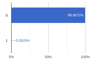
- As they train further continuously the fraud detection ML models, data professionals would like to set up an automatic check on data quality and be notified when there are huge discrepancies between
predicted_classandClassvalues. This is where Dataplex data quality could help the team.
Setup Data Quality Jobs
After setting up the data profiling scan we have seen that we still have no clear visibility on fluctuation between predicted_classes vs actual Class ratio. Our goal is to have a percentage of matched values between Class and predicted_classes more than 99.99 %. Any lower percentage would indicate that we would have to further train the ML model or add more features or use another model architecture.
You can use the following SQL query in BigQuery to check the percentage of matched values between Class and predicted_classes.
WITH RankedPredictions AS (
 SELECT
   class,
   ARRAY(
     SELECT AS STRUCT classes, scores
     FROM UNNEST(predicted_class.classes) classes WITH OFFSET AS pos
     JOIN UNNEST(predicted_class.scores) scores WITH OFFSET AS pos2
     ON pos = pos2
     ORDER BY scores DESC
     LIMIT 1
   )[OFFSET(0)].*
 FROM
   `<PROJECT_ID>.bootkon_raw_zone.data_predictions`
)

SELECT
 SUM(CASE WHEN class = CAST(highest_score_class AS STRING) THEN 1 ELSE 0 END) * 100.0 / COUNT(*)  AS PercentageMatch
FROM (
 SELECT
  class,classes AS highest_score_class
 FROM
   RankedPredictions
)
We will set up the Dataplex automatic data quality, which lets you define and measure the quality of your data. You can automate the scanning of data, validate data against defined rules, and log alerts if your data doesn’t meet quality requirements. You can manage data quality rules and deployments as code, improving the integrity of data production pipelines.
During the previous lab, we got started by using Dataplex data profiling rule recommendations to drive initial conclusions on areas of attention. Dataplex provides monitoring, troubleshooting, and Cloud Logging alerting that’s integrated with Dataplex auto data quality.
Conceptual Model
A data scan is a Dataplex job which samples data from BigQuery and Cloud Storage and infers various types of metadata. To measure the quality of a table using auto data quality, you create a DataScan object of type data quality. The scan runs on only one BigQuery table. The scan uses resources in a Google tenant project, so you don’t need to set up your own infrastructure. Creating and using a data quality scan consists of the following steps:
- Rule definition
- Rule execution
- Monitoring and alerting
- Troubleshooting
Lab Instructions
-
Go to the
Data profiling & quality section in the left hand menu of Dataplex. -
Click on
Create data quality scan -
Display Name:
bootkon-dquality-fraud-predictionfor example -
Optionally add a description. For example, “data quality scans for fraud detection predictions”
-
Leave the “Browse within Dataplex Lakes” option turned off
-
Click
BROWSE to filter on thedata_predictionsBigQuery table (Dataset:bootkon_raw_zone) -
SELECT data_predictionsBigQuery table -
Choose “Entire data” as the
Scope of the data profiling job -
Choose “All data” for
Sampling size -
Leave on the option “Publish results to BigQuery and Dataplex Catalog UI”
-
Choose On-demand as the scan schedule
-
Click
CONTINUE
Now let’s define quality rules. Click on the SQL Assertion Rule
- Choose
Accuracyas dimension - Rule name:
bootkon-dquality-ml-fraud-prediction - Description :
Regularly check the ML fraud detection prediction quality results - Leave the column name empty
- Provide the following SQL statement. Dataplex will utilize this to create a SQL clause of the form SELECT COUNT(*) FROM (sql statement) to return success/failure. The assertion rule is passed if the returned assertion row count is 0.
WITH RankedPredictions AS (
 SELECT
   class,
   ARRAY(
     SELECT AS STRUCT classes, scores
     FROM UNNEST(predicted_class.classes) classes WITH OFFSET AS pos
     JOIN UNNEST(predicted_class.scores) scores WITH OFFSET AS pos2
     ON pos = pos2
     ORDER BY scores DESC
     LIMIT 1
   )[OFFSET(0)].*,
 FROM
   `<PROJECT_ID>.bootkon_raw_zone.data_predictions`
)

SELECT
 SUM(CASE WHEN class = CAST(highest_score_class AS STRING) THEN 1 ELSE 0 END) * 100.0 / COUNT(*)  AS PercentageMatch
FROM (
 SELECT
   class,
   classes AS highest_score_class
 FROM
   RankedPredictions
)
   HAVING PercentageMatch <= 99.99
- Click
ADD - Click
CONTINUE RUN SCAN (The display name may take a moment to appear on the screen)- Monitor the job execution. Notice the job succeeded but the rule failed because our model accuracy percentage on the whole data predicted does not exceed the 99.99% threshold that we set
- You may need to choose
RUN NOW in order to see the results of thebootkon-dquality-fraud-predictiondata quality scan
Success
🎉 Congratulations ! 🚀
You’ve successfully completed the Data & AI Boot-Kon Dataplex lab! You’ve gained a solid understanding of Dataplex, creating lakes and zones, and adding assets from GCS and BigQuery.
You built data profiling and quality checks, exploring assets and setting up monitoring for fraud detection predictions. Even with the accuracy not yet at 99.99%, you’ve established monitoring for improvement – proactive data governance!
Bring on the next challenge – you’ve got this! 🚀
Conclusion
Development Workflow
First, start bootkon as if you were a participant (see Labs). Next, open this file in Cloud Shell:
bk-tutorial docs/book/contributing.md
Continue the next sections in the Cloud Shell tutorial.
Authenticate to GitHub
Cloud Shell editor supports authentication to GitHub via an interactive authentication flow. In this case, you just push your changes and a notification appears to guide you through this process. If you go this route, please continue with Set up git.
If, for some reason, this doesn’t work for you, you can use the following method:
Create SSH keys if they don’t exist yet (just hit return when it asks for passphrases):
test -f ~/.ssh/id_rsa.pub || ssh-keygen -t rsa
Display your newly created SSH key and add it to your GitHub account:
cat ~/.ssh/id_rsa.pub
Overwrite the remote URL to use the SSH protocol insead of HTTPS. Adjust the command in case you are working on your personal fork:
git remote set-url origin git@github.com:fhirschmann/bootkon.git
Set up git
git config --global user.name "John Doe"
git config --global user.email johndoe@example.com
Check your git config:
cat ~/.gitconfig
Pushing to GitHub
You can now commit changes and push them to GitHub. You can either use the version control of the Cloud Shell IDE (tree icon on the left hand side) or the command line:
git status
Set up your development environment
During the first lab, participants are asked to edit vars.sh. It is suggested to make a copy of this file and not touch the original in order not to accidently commit it to git.
First, make a copy:
cp vars.sh vars.local.sh
And edit it. It also runs on Argolis (for Google employees).
Next, source it:
. vars.local.sh
Note that the init script (bk) automatically loads vars.local.sh the next time and vars.local.sh takes presendence over vars.sh.
Reloading the tutorial
You can reload a lab on-the-fly by typing bk-tutorial followed by the lab markdown file into the terminal and pressing return. Let’s reload
this tutorial:
bk-tutorial docs/book/contributing.md
Working with mdbook
You can run mdbook and compile the book in Cloud Shell directly. First, install dependencies:
pip install jinja2 nbformat nbconvert
Next, run mdbook:
bk-mdbook
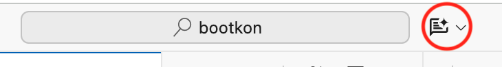
You can now read the book using Cloud Shell’s web preview by pressing the  button in Cloud Shell. Select Preview on port 8080. As soon as you change any of the markdown source files, mdbook will automatically reload it.
Authors
This version is based on a previous version by Wissem Khlifi.
The authors of Data & AI Bootkon are:
- Fabian Hirschmann (maintainer; main author)
- Cary Edwards (contributor)
- Daniel Holgate (contributor)
- Wissem Khlifi (original author)
Data & AI Bootkon received contributions from many people, including: